This record provides an overview of the NESP Marine and Coastal Hub small-scale study - Project 3.4 – Better Management of Catchment Runoff to Marine Receiving Environments in Northern Australia. For specific data outputs from this project, please see child records associated with this metadata. There are many catchments in northern Australia where increased catchment development is proposed. This is largely in the form of irrigation development, but also increased cattle stocking rates. Given the relatively low levels of such development in many catchments to date, there is a strong desire to maintain the integrity of coastal and marine receiving environments after the implementation of future developments. The baseline understanding of water quality in receiving marine environments and in the contributing catchments is very limited across much of northern Australia, making management and other development decisions very challenging. However, there are examples of intensive grazing and irrigation developments in northern Australia, e.g. in the Lower Burdekin Delta, adjacent to the Great Barrier Reef coastline, where lessons can be learnt to fast-track understandings and management and set testable hypotheses about the potential impacts of development in other northern catchments. This project aims to take advantage of these existing examples to improve the quality of decision-making around the impact of terrestrial runoff on the marine environment, providing a template for decision-makers. Planned Outputs • River plume modelling [spatial dataset] • Estimated river plume sediment and Chlorophyll loads [modelling dataset] • Mangrove extents remote sensing [modelling dataset] • Primary production response to nutrients in estuaries [experimental dataset • Final technical report with analysed data and a short summary of recommendations for policy makers of key findings [written]

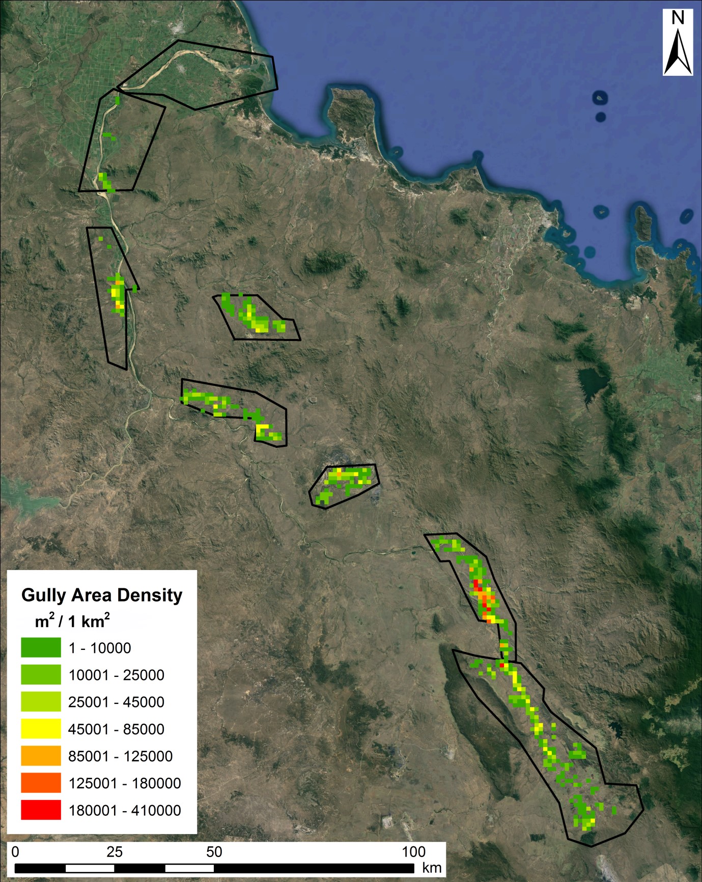
This dataset contains maps of alluvial and hillslope gullies across blocks of lidar covering portions of the Burdekin Catchment. This project is an expansion of the detailed gully mapping and assessment undertaken previously as part of NESP TWQ Project 5.10 (Daley et al., 2021), using newly available lidar as well as some older data not previously used. The gully polygons were generated using methods developed in the NESP TWQ 5.10 project for the extraction of gullies from lidar. Lidar is detailed topographic data collected from aircraft using an airborne laser scanning system. Methods: Lidar mapping and Gully Assessment SON3352211, December 2023. This project should be considered as the first step of a ‘prospecting’ effort, whereby high yielding high priority gullies are identified. Further investigations will be required (including on ground inspection) to firm up the prioritisation of gullies for rehabilitation. In all, gully mapping has been conducted across 1625 km2 (Figure 1). This is the area of lidar derived DEMs adjoining the areas within the Burdekin previously analysed by Daley et al. (2021) (Figure 1). This report briefly describes the generation of a new gully mapping dataset covering the 8 lidar blocks of the study area. Daley et al. (2021) provide a comprehensive description and discussion of the methods used below. Two small departures from the methods outlined therein have been adopted here. Firstly, the production of data layers was reordered, such that analyses that were previously restricted to just areas mapped as eroded landforms (i.e. PAE and Bare Soil described below) were here undertaken across the whole landscape, with the presence of high values for these metrics being used to identify areas for further investigation. This is a reversal (in a sense) of the approach used by Daley et al, who mapped all “gully like” features and then used PAE and Bare Soil metrics to distinguish actual gullies from features merely gully like. Here the approach has been to only search for (and map) gullies within areas of high PAE and Bare Soil. The second difference adopted here has been to define gully boundaries using two separate techniques for all observed gullies. In Daley et al, the choice of technique used to define the gully boundary was based on interrogation of general landscape slope, with 2% selected as a threshold separating areas where the Multi-direction hillshade (MDHS) approach was used from areas where the Mean Digital Elevation Model of Difference (Mean DoD) method was used. Early experimentation as part of this project found that this threshold method was occasionally unsatisfactory, as there were instances across all slope classes where the alternative approach provided the better representation of gully outline. In general, it was found that the MDHS method worked best where the gully had a more open form, which generally, but not always, occurred in areas of lower slope. Likewise it was found that the Mean DoD method worked best for linear or more reticulated forms, which generally but not always occurred in areas of higher slope. Examples of where the later did not apply is when an open form gully has mostly stabilised and revegetated, then re-incised, with the early phases of this re-incision taking the form of inset, more or less linear and/or reticulated gullying. To avoid the large amount of manual editing required where an inappropriate method was applied, it was found to be more parsimonious to run both techniques across all gullies, then select the approach which provided the best definition of gully boundary, requiring the least amount of manual digitising. 1. Mosaiced Digital Elevation Models (DEM) One kilometre square DEMs were obtained from Geoscience Australia’s ELVIS portal (https://elevation.fsdf.org.au/) and mosaiced into 8 larger DEMs, each covering one of the 8 non-contiguous areas shown in Figure 1. The DEM data was used to define gully margins and derive the Potential Active Erosion (PAE) layers. As depicted in figure 1, the spatial resolution of the DEMs of blocks 1 to 5 is 0.5 m and blocks 6 to 8 is 1 m. 2. Potential Active Erosion (PAE) The PAE method developed (and wholly described) by Daley et al. 2021 is an index of landscape curvature or crenulation. The index uses a measure of surface roughness derived using a log-transformed standard deviation of terrain curvature. Most erosion activity indicators correspond to areas exhibiting high values of surface roughness, including fluting, rilling, block collapse, slumping and exposed tree roots. As erosion activity decreases, slopes relax to more diffuse forms with lower roughness. Terrain roughness was measured as the local standard deviation of curvature in a 3 m kernel window, assessed from total, plan and profile curvatures. As roughness was highly skewed, with most values approximating zero, the data was log-transformed for ease of interpretation. Planform, profile and total curvatures were calculated within a 9-cell (3 x 3 m) neighbourhood using the ArcGIS curvature tool following the method of Moore et al. (1991) and Zevenbergen and Thorne (1987). All three types of curvature were evaluated to generate roughness indices following current literature as the log-normalised standard deviation of curvature (Korzeniowska et al. 2018; Patton et al. 2018). As standard deviation values in a 3 m cell kernel size were strongly right skewed, values were transformed using a base-10 logarithm function to normalise the distribution for ease of interpretation. Following Daley et al., a threshold log-normalised standard deviation of curvature value of 1.8 was chosen to define areas of PAE. 3. Bare Soil Baresoil was determined using PlanetScope Analytic data, with all scenes collected soon after the end of the 2022-2023 wet season. PlanetScope provides 4-band multi-spectral ortho scene data for analytic and visual applications. The provided product is orthorectified, radiometrically calibrated into top-of-atmosphere radiance data and then atmospherically corrected to surface reflectance, resampled to 3 m (Planet Team, 2020). This data was specifically selected for 90% coverage in a given acquisition. Additional data from neighbouring days were selected to fill in any gaps for complete coverage. Following data acquisition, scenes were mosaiced in a GIS to provide a continuous coverage dataset across the 8 study areas. Bare soil was derived from the PlanetScope imagery using the modified secondary soil-adjusted vegetation index (MSAVI2), Qi et al. (1994). MSAVI2 was selected as the most appropriate vegetation index for the region for its capacity to separate vegetation signatures in areas where vegetation cover is low, or features a high degree of exposed soil surface, and has the benefit over other soil-adjusted vegetation indices in that it does not require the calculation of a soil-brightness correction factor. MSAVI2 was developed iteratively by Qi et al. (1994) to determine the per-pixel difference of the red band reflectance value against the near infrared band, using the following equation: MSAVI2 = (2×NIR + 1 - √((2×NIR+1)^2 - 8×(NIR-RED)))/2 This yields an output of vegetation greenness with values ranging from -1 to +1. Following Daley et al, a threshold of 0.35 was used to identify bare soils. 4. Gully Mapping Gully boundaries were produced using the aforementioned Multi-direction hillshade (MDHS) and Mean DEMoD automated geomorphic mapping algorithms. For MDHS, the hillshade tool in ArcGIS Spatial Analyst is used iteratively, with the sun angle set at 15 degrees and passed through the six azimuths (0, 60, 120, 180, 240, 300 degrees). The output rasters of the hillshades are then mosaiced and areas <= 55 (i.e., lowest greyscale intensity value) are selected. These values are generally a function of slope and aspect for any given cell, but in this case, they are viewed as the amount of shadow generated by the moving sun. At each azimuth, the boundary of an eroded land form (ELF) is shadowed perpendicular to the direction of light. By merging the six hillshades, the boundary of a given gully is accurately extracted (see cross section C in Figure 2). In certain instances when a feature has low or diffuse walls, or a broad floor, the centre of the gully may not be shadowed, hence the centre of these gullies are filled to create a clean boundary. The Mean DoD method identifies abrupt changes in elevation assuming such changes equate to steep slopes on the walls of gullies. The mean focal statistic function was used with a circular window having a kernel radius of 25m. 5. Gully Distribution The area covered by the gully mapping polygons was divided into a 1 km x 1 km grid. One or two square kilometres is assumed to represent the size of an area that could be managed as one site containing multiple gullies. For each polygon the total area of mapped gullies contained within has been calculated (Figure 4) and plotted as a heat map. This is to facilitate prioritisation based on combined gully area within close proximity, rather than based on the size of any single gully. Limitations of the data: The funding for this project necessitated different priorities and a different scope of works than that of NESP TWQ 5.10, and consequently the set of derived gully metrics in this project is a subset of those in NESP TWQ 5.10. This dataset is specifically a selection of large prospectively high yielding gullies mapped as preparatory work towards future landscape repair programs which require detailed maps of gully extent in order to enable prioritisation and planning of works. This project should be considered as the first step of a ‘prospecting’ effort, whereby high yielding high priority gullies are identified. Further investigations will be required (including on ground inspection) to firm up the prioritisation of gullies for rehabilitation. Format of the data: Two shapefiles The gully mapping dataset consists of the shapefile – ‘Gully Mapping - Project SON3352211.shp’. The shapefile contains 1713 gully polygons. The gully density dataset consists of the shapefile – ‘Gully Density One km Grid - Project SON3352211.shp’. The shapefile contains 467 one km grid square polygons. Data dictionary: Gully mapping shapefile (Gully Mapping - Project SON3352211.shp) attribute table fields X - X co-ordinate of gully polygon centre point Y - Y co-ordinate of gully polygon centre point Gully_Code - Gully polygon ID number BaseData - DEM data acquisition name as stored in Geoscience Australia’s ELVIS data portal CellSize - Raster cell size (m) of base DEM data G_Area_m2 - Gully polygon area (m2) BS_Area_m2 - Area of bare soil as derived from Planet Scope imagery (m2) within gully polygons PCT_BS - Bare soil area as percentage of gully polygon area PAEArea_m2 - Area of Potential Active Erosion (m2) within gully polygon PCT_PAE - Potential Active Erosion area as percentage of gully polygon area Gully density shapefile (Gully Density One km Grid - Project SON3352211.shp) attribute table fields X - X co-ordinate of one km grid square polygon centre point Y - Y co-ordinate of one km grid square polygon centre point GulArea_m2 - Area of gully polygon within one km grid square (m2) References: Daley, J., Stout, J.C., Curwen, G., Brooks, A.P. and Spencer, J. (2021) Development and application of automated tools for high resolution gully mapping and classification from lidar data. Report to the National Environmental Science Program. Reef and Rainforest Research Centre Limited, Cairns (169pp.). Korzeniowska, K., Pfeifer, N., & Landtwing, S. (2018). Mapping gullies, dunes, lava fields, and landslides via surface roughness. Geomorphology, 301, 53-67 Moore, I.D., Grayson, R.B., Landson, A.R. (1991) Digital Terrain Modelling: A Review of Hydrological, Geomorphological, and Biological Applications. Hydrological Processes 5: 3–30. Patton, N. R., Lohse, K. A., Godsey, S. E., Crosby, B. T., & Seyfried, M. S. (2018). Predicting soil thickness on soil mantled hillslopes. Nature communications, 9(1), 3329. Planet Team (2020). Planet Imagery Product Specification. San Francisco, CA. https://developers.planet.com/changelog/2020/Jun/17/imagery/2020-06-17/ Qi, J., Chehbouni, A., Huete, A.R., Kerr, Y. H., and Sorooshian, S. (1994). A Modified Soil Adjusted Vegetation Index. Remote Sensing of Environment. 48: 119-126 Zeverbergen, L.W., Thorne, C.R. (1987) Quantitative Analysis of Land Surface Topography. Earth Surface Processes and Landforms 12: 47–56. Map Description: The map layers show polygons of gully areas in the Burdekin Catchment which have been mapped and analysed to identify gullies with areas of potential active erosion. The second heat map layer shows square areas at 1 km x 1 km resolution which identify areas of high density gullies with potential active erosion. eAtlas Processing: The original data were provided as two shapefiles. No modifications to the underlying data were performed and the data package are provided as submitted. Location of the data: This dataset is filed in the eAtlas enduring data repository at: data\\custodian\2022-2029-Other\QLD_GU_Lidar-Mapping-Gully-Assessment_2023